Over the past few decades, Computer Science has become increasingly prevalent in finance and economics. Top financial firms are relying on computers to deliver results. For example, JP Morgan, Chase, and Barclays depend on supercomputers to estimate a stock portfolio’s risk or predict an asset’s future value. How do they do this?
In this article, I will be exploring how computers analyze sentiment and utilize machine learning to maximize return on investments.
Sentiment Analysis
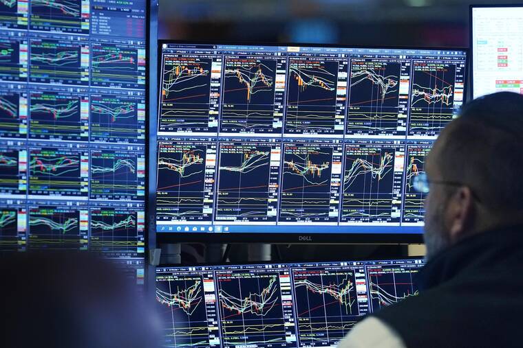
The market has shifted from investing on instinct to instilling trust in computer programs. The days of traders frantically buying and selling stocks on the trading floor are waning. Replacing floor traders are quantitative analysts or quant for short. Quants develop computer algorithms with a heavy emphasis on math to execute trades and forecast the future performance of a stock.
Recognizing the shift in the market, Dow Jones has developed a lexicon to allow computers to easily analyze how a stock might move. Another word for lexicon is dictionary. The Dow Jones Lexicon (DJL) collects financial news and converts it into a language that computers understand. Moreover, the DJL has six different dictionaries, all created by Bill McDonald, a professor of finance at the University of Notre Dame. However, financial firms can create their own dictionaries to suit their specific needs.
When a computer is equipped with a lexicon it can recognize positive news from negative. This then informs traders whether or not it would be wise to execute a trade for this stock.
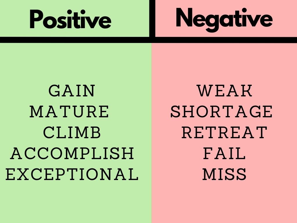
Below is a graphic depicting whether sentiment for a stock is bullish (positive) or bearish (negative)
Let’s analyze a news article to examine how the sentiment lexicon works. This article is from CNBC and was published on November 26, 2021, just days after scientists in South Africa discovered a new variant of COVID.
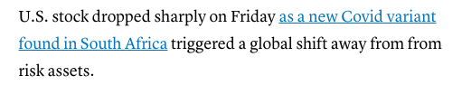
This is the opening line of the article. You will notice that one of the first words is “dropped.” A computer analyzing this snippet of text would categorize it into the negative section and decrease the sentiment score, indicating that the stock market is bearish. However, the placement of the word is also important. Keywords that are placed in headlines or the first few lines have more weight on the sentiment score than they would if they were buried in the body of the text.
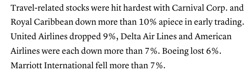
In this screenshot, you will notice keywords such as, “down,” “dropped,” “lost,” and “fell.” Again, these are words that the computer will interpret as negative thereby decreasing the sentiment score.
Now, how does this look on the computer end? It turns out that it is a relatively simple process. Creating a sentiment analysis program is achieved by the use of XML code. XML stands for extensible markup language and is closely related to HTML, however, it is not its own language. HTML describes how a document should appear while XML describes the data within the document. For example, in HTML there are tags that a programmer inserts to create certain objects. For example, the <h1> tag describes a heading of a website (h for heading; 1 for the first heading). Meanwhile, XML lets a programmer customize their code even further. For example, instead of creating a vaguely defined <h1> tag, XML allows the programmer to denote the tag as something like <stock> to make it clear as to what is being defined. This makes it easier to interpret code and cater to a business’s needs.
Note: the following code was compiled by sqlauthority.com
<SampleXML>
<Colors>
   <Color1>White</Color1>
   <Color2>Blue</Color2>
   <Color3>Black</Color3>
   <Color4 Special="Light">Green</Color4>
   <Color5>Red</Color5>
</Colors>
<Fruits>
   <Fruits1>Apple</Fruits1>
   <Fruits2>Pineapple</Fruits2>
   <Fruits3>Grapes</Fruits3>
   <Fruits4>Melon</Fruits4>
</Fruits>
</SampleXML>
In the example above, quants or traders would follow a similar format as pictured above, just changing the tags that are specific to an algorithm for sentiment analysis.
Sentiment analysis only scratched the surface of what computers can do on Wall Street. While I will not be able to discuss all, I will continue the article by discussing how Machine Learning comes into play in forecasting how the market will move.
Machine Learning
Machine Learning (ML) is a subcategory of Artificial Intelligence (AI) that gathers information for systems like Siri to make decisions. In this case, instead of Siri, it is computer algorithms. Read more about ML and AI in a previous post I created.
To have the highest chance of success, the computer has to undergo training. Four characteristics of stock are used for training: Its open price, high of the day, low of the day, and trading volume. The following data is from Microsoft stock.
| Date | Open | High | Low | Close | Adj Close | Volume |
| 1990-01-02 | 0.605903 | 0.616319 | 0.598090 | 0.616319 | 0.447268 | 53033600 |
| 1990-01-03 | 0.621528 | 0.626736 | 0.614583 | 0.619792 | 0.449788 | 113772800 |
| 1990-01-04 | 0.619792 | 0.638889 | 0.616319 | 0.638021 | 0.463017 | 125740800 |
| 1990-01-05 | 0.635417 | 0.638889 | 0.621528 | 0.622396 | 0.451678 | 69564800 |
| 1990-01-08 | 0.621528 | 0.631944 | 0.614583 | 0.631944 | 0.458607 | 58982400 |
Note: the following code was compiled by Analytics Vidhya
Normalizing
To make it easier for the computer to handle the data, it must be normalized meaning scaled between the values 0 and 1. This also decreases memory, allowing quicker results. The succeeding data is the same as above but just normalized.
| Date | Open | High | Low | Volume |
| 1990-01-02 | 0.000129 | 0.000105 | 0.000129 | 0.064837 |
| 1990-01-03 | 0.000265 | 0.000195 | 0.000273 | 0.144673 |
| 1990-01-04 | 0.000249 | 0.000300 | 0.000288 | 0.160404 |
| 1990-01-05 | 0.000386 | 0.000300 | 0.000334 | 0.086566 |
| 1990-01-08 | 0.000265 | 0.000240 | 0.000273 | 0.072656 |
The code below declares variables discussed above to enable the computer to later manipulate them.
#Set Target Variable
output_var = PD.DataFrame(df[‘Adj Close’])
#Selecting the Features
features = [‘Open’, ‘High’, ‘Low’, ‘Volume’]
To split data into a training set and a test set, the following code must be implemented.
#Splitting to Training set and Test set
timesplit= TimeSeriesSplit(n_splits=10)
for train_index, test_index in timesplit.split(feature_transform):
        X_train, X_test = feature_transform[:len(train_index)], feature_transform[len(train_index): (len(train_index)+len(test_index))]
        y_train, y_test = output_var[:len(train_index)].values.ravel(), output_var[len(train_index): (len(train_index)+len(test_index))].values.ravel()
The training set of data will be fed into a Machine Learning long short-term model (LSTM). An LSTM is an artificial recurrent neural network utilized to learn the stock’s pattern. After the pattern is learned, a predict function will be available to call.
#Process the data for LSTM
trainX =np.array(X_train)
testX =np.array(X_test)
X_train = trainX.reshape(X_train.shape[0], 1, X_train.shape[1])
X_test = testX.reshape(X_test.shape[0], 1, X_test.shape[1])
The way in which the data runs through the LSTM model is structured as such:
#Building the LSTM Model
lstm = Sequential()
lstm.add(LSTM(32, input_shape=(1, trainX.shape[1]), activation=’relu’, return_sequences=False))
lstm.add(Dense(1))
lstm.compile(loss=’mean_squared_error’, optimizer=’adam’)
plot_model(lstm, show_shapes=True, show_layer_names=True)
Finally, the data is ready to be trained.
#Model Training
history=lstm.fit(X_train, y_train, epochs=100, batch_size=8, verbose=1, shuffle=False)
Eросh  1/100
834/834  [==============================]  –  3s  2ms/steр  –  lоss:  67.1211
Eросh  2/100
834/834  [==============================]  –  1s  2ms/steр  –  lоss:  70.4911
Eросh  3/100
834/834  [==============================]  –  1s  2ms/steр  –  lоss:  48.8155
Eросh  4/100
834/834  [==============================]  –  1s  2ms/steр  –  lоss:  21.5447
Eросh  5/100
834/834  [==============================]  –  1s  2ms/steр
.
.
.
.
Eросh  95/100
834/834  [==============================]  –  1s  2ms/steр  –  lоss:  0.4542
Eросh  96/100
834/834  [==============================]  –  2s  2ms/steр  –  lоss:  0.4553
Eросh  97/100
834/834  [==============================]  –  1s  2ms/steр  –  lоss:  0.4565
Eросh  98/100
834/834  [==============================]  –  1s  2ms/steр  –  lоss:  0.4576
Eросh  99/100
834/834  [==============================]  –  1s  2ms/steр  –  lоss:  0.4588
Eросh  100/100
834/834  [==============================]  –  1s  2ms/steр  –  lоss:  0.4599
In the code above, you will notice that the data is fed through an epoch. One epoch signifies one cycle through the training of the data set. To properly train a data set, numerous epochs are used because each cycle can produce a different method to arrive at the solution. This enables the model to predict the movement of a stock quicker and more accurately. Greater accuracy is observed by the fact that the loss (error) decreases greatly over the course of training.
After the data is fed into 100 epochs, the model can reliably predict. This is achieved with the predict function.
#LSTM Prediction
y_pred= lstm.predict(X_test)
To assess its accuracy, plot the actual value of the stock and the predicted value.
#Predicted vs True Adj Close Value – LSTM
plt.plot(y_test, label=’True Value’)
plt.plot(y_pred, label=’LSTM Value’)
plt.title(“Prediction by LSTM”)
plt.xlabel(‘Time Scale’)
plt.ylabel(‘Scaled USD’)
plt.legend()
plt.show()
Output:
Remember, the y-axis is in terms of the normalized values discussed above.
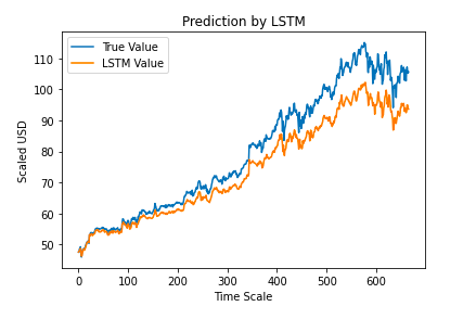
While the predicted values are not completely in line with the actual values, patterns in the stock are very similar. However, this is just the output of a basic LSTM network model. By creating a more advanced LSTM network or analyzing different patterns within the stock such as moving averages, predictions can become even closer to the actual values.

Clearly, computers are becoming increasingly ingrained within the financial community. Financial firms are depending on computers to deliver results. Sentiment analysis and machine learning are just a couple ways technology has been implemented within the stock market. It is still an evolving situation and the future will bring upon even more innovation in the field.
If you are interested in learning more about computer science visit its subject page on our site! There, you will find a plethora of resources to take advantage of.
References
https://www.wired.com/2010/12/ff-ai-flashtrading/?scrlybrkr=1c48305a
https://hbr.org/2000/07/explaining-xml
https://www.youtube.com/watch?v=KeLiQXqVgMI